Symmetric mean absolute percentage error

Statistical deviation and dispersion

Symmetric mean absolute percentage error (SMAPE or sMAPE) is an accuracy measure based on percentage (or relative) errors. It is usually defined as follows: where At is the actual value and Ft is the forecast value. The absolute difference between At and Ft is divided by half the sum of absolute values of the actual value At and the forecast value Ft. The value of this calculation is summed for every fitted point t and divided again by the number of fitted points n. The earliest reference to similar formula appears to be Armstrong (1985, p. 348) where it is called "adjusted MAPE" and is defined without the absolute values in denominator. It has been later discussed, modified and re-proposed by Flores (1986). Armstrong's original definition is as follows: The problem is that it can be negative (if ) or even undefined (if ). Therefore the currently accepted version of SMAPE assumes the absolute values in the denominator. In contrast to the mean absolute percentage error, SMAPE has both a lower bound and an upper bound. Indeed, the formula above provides a result between 0% and 200%. However a percentage error between 0% and 100% is much easier to interpret. That is the reason why the formula below is often used in practice (i.e. no factor 0.5 in denominator): In the above formula, if , then the t'th term in the summation is 0, since the percent error between the two is clearly 0 and the value of is undefined. One supposed problem with SMAPE is that it is not symmetric since over- and under-forecasts are not treated equally. This is illustrated by the following example by applying the second SMAPE formula: * Over-forecasting: At = 100 and Ft = 110 give SMAPE = 4.76% * Under-forecasting: At = 100 and Ft = 90 give SMAPE = 5.26%. However, one should only expect this type of symmetry for measures which are entirely difference-based and not relative (such as mean squared error and mean absolute deviation). There is a third version of SMAPE, which allows to measure the direction of the bias in the data by generating a positive and a negative error on line item level. Furthermore it is better protected against outliers and the bias effect mentioned in the previous paragraph than the two other formulas.The formula is: A limitation to SMAPE is that if the actual value or forecast value is 0, the value of error will boom up to the upper-limit of error. (200% for the first formula and 100% for the second formula). Provided the data are strictly positive, a better measure of relative accuracy can be obtained based on the log of the accuracy ratio: log(Ft / At)This measure is easier to analyse statistically, and has valuable symmetry and unbiasedness properties. When used in constructing forecasting models the resulting prediction corresponds to the geometric mean (Tofallis, 2015). (Wikipedia).

Percent Uncertainty In Measurement

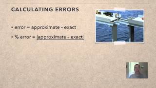
This video tutorial provides a basic introduction into percent uncertainty. It also discusses topics such as estimated uncertainty, absolute uncertainty, and relative uncertainty. This video provides an example explaining how to calculate the percent uncertainty in the volume of the sphe

From playlist New Physics Video Playlist

IAML8.21 Mean absolute error (MAE)

From playlist Generalization and Evaluation

Error and Percentage Error

From playlist a. Numbers and Measurement

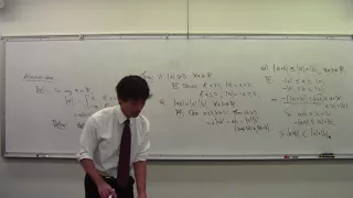
Math 101 091117 Introduction to Analysis 05 Absolute Value

Absolute value: definition. Notion of distance. Properties of the absolute value: proofs. Triangle inequality

From playlist Course 6: Introduction to Analysis (Fall 2017)

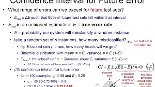
IAML8.7 Confidence interval for generalization

From playlist Generalization and Evaluation

Lesson: Calculate a Confidence Interval for a Population Proportion

This lesson explains how to calculator a confidence interval for a population proportion.

From playlist Confidence Intervals

Absolute Extrema

http://mathispower4u.wordpress.com/

From playlist Differentiation Application - Absolute Extrema

What is the definition of absolute value

http://www.freemathvideos.com In this video playlist you will learn how to solve and graph absolute value equations and inequalities. When working with absolute value equations and functions it is important to understand that the absolute value symbol represents the absolute distance from

From playlist Solve Absolute Value Equations

Linear Algebra 9.2 The Power Method

My notes are available at http://asherbroberts.com/ (so you can write along with me). Elementary Linear Algebra: Applications Version 12th Edition by Howard Anton, Chris Rorres, and Anton Kaul A. Roberts is supported in part by the grants NSF CAREER 1653602 and NSF DMS 2153803.

From playlist Linear Algebra

7. Value At Risk (VAR) Models

MIT 18.S096 Topics in Mathematics with Applications in Finance, Fall 2013 View the complete course: http://ocw.mit.edu/18-S096F13 Instructor: Kenneth Abbott This is an applications lecture on Value At Risk (VAR) models, and how financial institutions manage market risk. License: Creative

From playlist MIT 18.S096 Topics in Mathematics w Applications in Finance

CSE 519 -- Lecture 19, Fall 2020

From playlist CSE 519 -- Fall 2020

[LIVE] Rasa Reading Group: Grokking: Generalisation beyond overfitting on small algorithmic datasets

The Reading Group is back for special edition! Join us as we read an ML paper together live. This week we'll be reading the paper "Grokking: Generalisation beyond overfitting on small algorithmic datasets" by Alethea Power, Yuri Burda, Harri Edwards, Igor Babuschkin & Vedant Misra from Ope

From playlist Rasa Reading Group

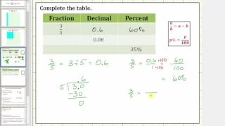
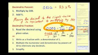
Percent Intro and Basic Percent, Fraction, Decimal Conversions (No Calculator)

This video defines a percent and explains how to perform basic percent, fraction, and decimal conversions.

From playlist Introduction to Percentages

Analyze Phase In Six Sigma | Six Sigma Green Belt Training

The fourth lesson of the Lean Six Sigma Green Belt Course offered by Simplilearn. This lesson will cover the details of the analyze phase. In the Lean Six Sigma process, you begin with the define phase where you define the problem and then the current process performance is measured. Next

From playlist Six Sigma Training Videos [2022 Updated]

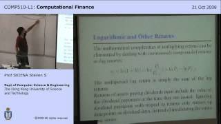
Lecture 13 - Financial Time Series Data

This is Lecture 13 of the COMP510 (Computational Finance) course taught by Professor Steven Skiena [http://www.cs.sunysb.edu/~skiena/] at Hong Kong University of Science and Technology in 2008. The lecture slides are available at: http://www.algorithm.cs.sunysb.edu/computationalfinance/pd

From playlist COMP510 - Computational Finance - 2007 HKUST

Lec 15 | MIT 6.00SC Introduction to Computer Science and Programming, Spring 2011

Lecture 15: Statistical Thinking Instructor: John Guttag View the complete course: http://ocw.mit.edu/6-00SCS11 License: Creative Commons BY-NC-SA More information at http://ocw.mit.edu/terms More courses at http://ocw.mit.edu

From playlist MIT 6.00SC Introduction to Computer Science and Programming

Introduction to Laplacian Linear Systems for Undirected Graphs - John Peebles

Computer Science/Discrete Mathematics Seminar II Topic: Introduction to Laplacian Linear Systems for Undirected Graphs Speaker: John Peebles Affiliation: Member, School of Mathematics Date: February 23, 2021 For more video please visit http://video.ias.edu

From playlist Mathematics

Measure Phase In Six Sigma | Six Sigma Training Videos

🔥 Enrol for FREE Six Sigma Course & Get your Completion Certificate: https://www.simplilearn.com/six-sigma-green-belt-basics-skillup?utm_campaign=SixSigma&utm_medium=DescriptionFirstFold&utm_source=youtube Introduction to Measure Phase: The Measure phase is the second phase in a six sigm

From playlist Six Sigma Training Videos [2022 Updated]

A (Potential) Finite-Time Singularity and Thermalization in the 3D Axisymmetric... by Rahul Pandit

DISCUSSION MEETING : STATISTICAL PHYSICS OF COMPLEX SYSTEMS ORGANIZERS : Sumedha (NISER, India), Abhishek Dhar (ICTS-TIFR, India), Satya Majumdar (University of Paris-Saclay, France), R Rajesh (IMSc, India), Sanjib Sabhapandit (RRI, India) and Tridib Sadhu (TIFR, India) DATE : 19 December

From playlist Statistical Physics of Complex Systems - 2022

Introduction to Percent

http://mathispower4u.wordpress.com/

From playlist Percentages

Symmetric mean absolute percentage error

Related pages