Response modeling methodology

Nonlinear functional analysis | Statistical models | Transformation (function) | Regression models

Response modeling methodology (RMM) is a general platform for statistical modeling of a linear/nonlinear relationship between a response variable (dependent variable) and a linear predictor (a linear combination of predictors/effects/factors/independent variables), often denoted the linear predictor function. It is generally assumed that the modeled relationship is monotone convex (delivering monotone convex function) or monotone concave (delivering monotone concave function). However, many non-monotone functions, like the quadratic equation, are special cases of the general model. RMM was initially developed as a series of extensions to the original inverse Box–Cox transformation: where y is a percentile of the modeled response, Y (the modeled random variable), z is the respective percentile of a and λ is the Box–Cox parameter. As λ goes to zero, the inverse Box–Cox transformation becomes: an exponential model. Therefore, the original inverse Box-Cox transformation contains a trio of models: linear (λ = 1), power (λ ≠ 1, λ ≠ 0) and exponential (λ = 0). This implies that on estimating λ, using sample data, the final model is not determined in advance (prior to estimation) but rather as a result of estimating. In other words, data alone determine the final model. Extensions to the inverse Box–Cox transformation were developed by Shore (2001a) and were denoted Inverse Normalizing Transformations (INTs). They had been applied to model monotone convex relationships in various engineering areas, mostly to model physical properties of chemical compounds (Shore et al., 2001a, and references therein). Once it had been realized that INT models may be perceived as special cases of a much broader general approach for modeling non-linear monotone convex relationships, the new Response Modeling Methodology had been initiated and developed (Shore, 2005a, 2011 and references therein). The RMM model expresses the relationship between a response, Y (the modeled random variable), and two components that deliver variation to Y: * The linear predictor function, LP (denoted η): where {X1,...,Xk} are regressor-variables (“affecting factors”) that deliver systematic variation to the response; * Normal errors, delivering random variation to the response. The basic RMM model describes Y in terms of the LP, two possibly correlated zero-mean normal errors, ε1 and ε2 (with correlation ρ and standard deviations σε1 and σε2, respectively) and a vector of parameters {α,λ,μ} (Shore, 2005a, 2011): and ε1 represents uncertainty (measurement imprecision or otherwise) in the explanatory variables (included in the LP). This is in addition to uncertainty associated with the response (ε2). Expressing ε1 and ε2 in terms of standard normal variates, Z1 and Z2, respectively, having correlation ρ, and conditioning Z2 | Z1 = z1 (Z2 given that Z1 is equal to a given value z1), we may write in terms of a single error, ε: where Z is a standard normal variate, independent of both Z1 and Z2, ε is a zero-mean error and d is a parameter. From these relationships, the associated RMM quantile function is (Shore, 2011): or, after re-parameterization: where y is the percentile of the response (Y), z is the respective standard normal percentile, ε is the model's zero-mean normal error with constant variance, σ, {a,b,c,d} are parameters and MY is the response median (z = 0), dependent on values of the parameters and the value of the LP, η: where μ (or m) is an additional parameter. If it may be assumed that cz<<η, the above model for RMM quantile function can be approximated by: The parameter “c” cannot be “absorbed” into the parameters of the LP (η) since “c” and LP are estimated in two separate stages (as expounded below). If the response data used to estimate the model contain values that change sign, or if the lowest response value is far from zero (for example, when data are left-truncated), a location parameter, L, may be added to the response so that the expressions for the quantile function and for the median become, respectively: (Wikipedia).

Data Modeling Tutorial | Data Modeling for Data Warehousing | Data Warehousing Tutorial | Edureka

***** Data Warehousing & BI Training: https://www.edureka.co/data-warehousing-and-bi ***** Data modeling is a process used to define and analyze data requirements needed to support the business processes within the scope of corresponding information systems in organizations. Therefore, th

From playlist Data Warehousing Tutorial Videos

Fourier Series: Modeling Nature

An intuitive means of understanding the power of Fourier series in modeling nature, to place Fourier series in a physical context for students being introduced to the material. A non-technical, qualitative exploration into applications of Fourier Series. 0:17 Ancient Greek theory of celes

From playlist Data Science

What is Curve Fitting Toolbox? - Curve Fitting Toolbox Overview

Get a Free Trial: https://goo.gl/C2Y9A5 Get Pricing Info: https://goo.gl/kDvGHt Ready to Buy: https://goo.gl/vsIeA5 Fit curves and surfaces to data using regression, interpolation, and smoothing using Curve Fitting Toolbox. For more videos, visit http://www.mathworks.com/products/curvefi

From playlist Math, Statistics, and Optimization

What is Math Modeling? Video Series Part 6: Analysis

By the time you’ve reached the analysis step of the math modeling process, you’ve built a mathematical model -congratulations! Now it’s time to analyze and assess the quality of the model. In this step and number six in this seven-part series, modelers take an honest look at the body of wo

From playlist M3 Challenge

Principal Component Analysis

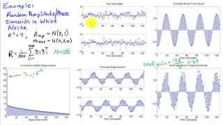
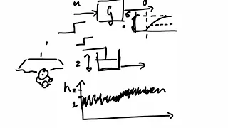
http://AllSignalProcessing.com for more great signal processing content, including concept/screenshot files, quizzes, MATLAB and data files. Representing multivariate random signals using principal components. Principal component analysis identifies the basis vectors that describe the la

From playlist Random Signal Characterization

Tony Lelievre (DDMCS@Turing): Coarse-graining stochastic dynamics

Complex models in all areas of science and engineering, and in the social sciences, must be reduced to a relatively small number of variables for practical computation and accurate prediction. In general, it is difficult to identify and parameterize the crucial features that must be incorp

From playlist Data driven modelling of complex systems

Causal Behavioral Modeling Framework - Discrete Choice Modeling of Consumer Demand

There are increasing demands for "causal ML models" of the agent behaviors, which enable us to unbox the complex black-box models and make inferences or do proper counterfactual simulations. Many applications (especially in Marketing) intrinsically call for measurement of the causal impact

From playlist Fundamentals of Machine Learning

05c Machine Learning: Feature Selection

Lecture on methods for feature selection for machine learning workflows. Follow along with the demonstration workflows in Python: o. Feature Selection / Ranking: https://github.com/GeostatsGuy/PythonNumericalDemos/blob/master/SubsurfaceDataAnalytics_Feature_Ranking.ipynb Subsurface Mach

From playlist Machine Learning

B27 Introduction to linear models

Now that we finally now some techniques to solve simple differential equations, let's apply them to some real-world problems.

From playlist Differential Equations

Step testing

We apply nonlinear curve fitting and linear regression to the problem of identifying the parameters of a model from responses over time

From playlist Parameter estimation

20 Data Analytics: Decision Tree

Lecture on decision tree-based machine learning with workflows in R and Python and linkages to bagging, boosting and random forest.

From playlist Data Analytics and Geostatistics

🔥Agile Scrum Full Course 2022 | Agile Scrum Master Training | Agile Tutorial | Simplilearn

🔥Certified ScrumMaster (CSM) Certification Training Course: https://www.simplilearn.com/agile-and-scrum/csm-certification-training?utm_campaign=AgileScrum2022-iCPkodTfcjU&utm_medium=DescriptionFirstFold&utm_source=youtube 🔥Certified Scrum Product Owner (CSPO) Certification Training: https

From playlist Simplilearn Live

Intro to Scikit-learn

Course: Intro to Scikit-learn Sept 17, 2020 Scikit-Learn Demonstration Demonstration of scikit learn for machine learning. In this workflow we demonstrate the plug and play nature of scikit learn machine learning models. For an unconventional dataset we demonstrate the following steps: 1.

From playlist daytum Free Webinar Series

11 Machine Learning: k-Nearest Neighbors

Lecture on k-nearest neighbor for machine learning prediction. Including more discussion on hyperparameters and variance-bias trade-off. Follow along with the demonstration workflow: https://github.com/GeostatsGuy/PythonNumericalDemos/blob/master/SubsurfaceDataAnalytics_kNearestNeighbour.

From playlist Machine Learning

Thomas Hudson - Multiscale Modeling - IPAM at UCLA

Recorded 17 March 2023. Thomas Hudson of the University of Warwick presents "Multiscale Modeling" at IPAM's New Mathematics for the Exascale: Applications to Materials Science Tutorials. Learn more online at: http://www.ipam.ucla.edu/programs/workshops/new-mathematics-for-the-exascale-appl

From playlist 2023 New Mathematics for the Exascale: Applications to Materials Science Tutorials

18 Machine Learning: Conclusion

Final lecture with the take-aways from the Subsurface Machine Learning course to help you succeed with machine learning for spatial, subsurface applications.

From playlist Machine Learning

CS472 Lecture 2: ICU operations, surveys, epidemiological models

From playlist CS472: Data science and AI for COVID-19

DevOps Methodology | DevOps Tutorial For Beginners | DevOps Tutorial | Simplilearn

🔥DevOps Engineer Master Program (Discount Code: YTBE15): https://www.simplilearn.com/devops-engineer-masters-program-certification-training?utm_campaign=DevOpsMethodology-HJhq6MaXcVQ&utm_medium=Descriptionff&utm_source=youtube 🔥Post Graduate Program In DevOps: https://www.simplilearn.com/

From playlist DevOps Tutorial For Beginners 🔥 | Simplilearn [Updated]

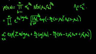
(ML 16.7) EM for the Gaussian mixture model (part 1)

Applying EM (Expectation-Maximization) to estimate the parameters of a Gaussian mixture model. Here we use the alternate formulation presented for (unconstrained) exponential families.

From playlist Machine Learning

Agile Scrum Full Course In 4 Hours | Agile Scrum Master Training | Agile Training Video |Simplilearn

🔥Certified ScrumMaster® (CSM) Certification Training Course: https://www.simplilearn.com/agile-and-scrum/csm-certification-training?utm_campaign=ASM-VFQtSqChlsk&utm_medium=DescriptionFirstFold&utm_source=youtube 🔥Certified Scrum Product Owner (CSPO) Certification Training: https://www.sim

From playlist Agile Scrum Master Training Videos [2022 Updated]

Response modeling methodology

Related pages