Coefficient diagram method

Control theory | Polynomials

In control theory, the coefficient diagram method (CDM) is an algebraic approach applied to a polynomial loop in the parameter space, where a special diagram called a "coefficient diagram" is used as the vehicle to carry the necessary information, and as the criterion of good design. The performance of the closed loop system is monitored by the coefficient diagram. The most considerable advantages of CDM can be listed as follows: 1. * The design procedure is easily understandable, systematic and useful. Therefore, the coefficients of the CDM controller polynomials can be determined more easily than those of the PID or other types of controller. This creates the possibility of an easy realisation for a new designer to control any kind of system. 2. * There are explicit relations between the performance parameters specified before the design and the coefficients of the controller polynomials as described in. For this reason, the designer can easily realize many control systems having different performance properties for a given control problem in a wide range of freedom. 3. * The development of different tuning methods is required for time delay processes of different properties in PID control. But it is sufficient to use the single design procedure in the CDM technique. This is an outstanding advantage. 4. * It is particularly hard to design robust controllers realizing the desired performance properties for unstable, integrating and oscillatory processes having poles near the imaginary axis. It has been reported that successful designs can be achieved even in these cases by using CDM. 5. * It is theoretically proven that CDM design is equivalent to LQ design with proper state augmentation. Thus, CDM can be considered an ‘‘improved LQG’’, because the order of the controller is smaller and weight selection rules are also given. It is usually required that the controller for a given plant should be designed under some practical limitations.The controller is desired to be of minimum degree, minimum phase (if possible) and stable. It must have enough bandwidth and power rating limitations. If the controller is designed without considering these limitations, the robustness property will be very poor, even though the stability and requirements are met. CDM controllers designed while considering all these problems is of the lowest degree, has a convenient bandwidth and results with a unit step time response without an overshoot. These properties guarantee the robustness, the sufficient damping of the disturbance effects and the low economic property. Although the main principles of CDM have been known since the 1950s, the first systematic method was proposed by . He developed a new method that easily builds a target characteristic polynomial to meet the desired time response. CDM is an algebraic approach combining classical and modern control theories and uses polynomial representation in the mathematical expression. The advantages of the classical and modern control techniques are integrated with the basic principles of this method, which is derived by making use of the previous experience and knowledge of the controller design. Thus, an efficient and fertile control method has appeared as a tool with which control systems can be designed without needing much experience and without confronting many problems. Many control systems have been designed successfully using CDM. It is very easy to design a controller under the conditions of stability, time domain performance and robustness. The close relations between these conditions and coefficients of the characteristic polynomial can be simply determined. This means that CDM is effective not only for control system design but also for controller parameters tuning. (Wikipedia).

How to find correlation in Excel with the Data Analysis Toolpak

Click this link for more information on correlation coefficients plus more FREE Excel videos and tips: http://www.statisticshowto.com/what-is-the-pearson-correlation-coefficient/

From playlist Regression Analysis

Scatterplots, Part 3: The Formula Behind the Correlation Coefficient

We use the Scatterplots & Correlation app to explain the formula behind the correlation coefficient. The app allows you to find and plot the z-scores, showing the 4 quadrants in which points on the scatterplot can fall.

From playlist Chapter 3: Relationships between two variables

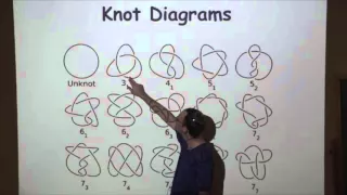
Estimate the Correlation Coefficient Given a Scatter Plot

This video explains how to estimate the correlation coefficient given a scatter plot.

From playlist Performing Linear Regression and Correlation

Scatterplots, Part 2: The Correlation Coefficient

From playlist Chapter 3: Relationships between two variables

Graphing Equations By Plotting Points - Part 2

This video shows how to graph equations by plotting points. Part 2 of 2 http://www.mathispower4u.yolasite.com

From playlist Graphing Various Functions

Graphing Equations By Plotting Points - Part 1

This video shows how to graph equations by plotting points. Part 1 of 2 http://www.mathispower4u.yolasite.com

From playlist Graphing Various Functions

What are the key points to trigonometric graphs

👉 Learn the basics of graphing trigonometric functions. The graphs of trigonometric functions are cyclical graphs which repeats itself for every period. To graph the parent graph of a trigonometric function, we first identify the critical points which includes: the x-intercepts, the maximu

From playlist How to Graph Trigonometric Functions

Phase shifts of trigonometric functions

From playlist How to Graph Trigonometric Functions

Speech and Audio Processing 4: Speech Coding I - Professor E. Ambikairajah

Speech and Audio Processing Speech Coding - Lecture notes available from: http://eemedia.ee.unsw.edu.au/contents/elec9344/LectureNotes/

From playlist ELEC9344 Speech and Audio Processing by Prof. Ambikairajah

Using composition of inverses using triangles

👉 Learn how to evaluate an expression with the composition of a function and a function inverse. Just like every other mathematical operation, when given a composition of a trigonometric function and an inverse trigonometric function, you first evaluate the one inside the parenthesis. We

From playlist Evaluate a Composition of Inverse Trigonometric Functions

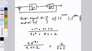
Simulation of systems with dead time Lecture 2019-02-27

Systems with dead time make it hard to do closed loop simulations. I cover a couple of ways to handle this. The video showing only the closed loop simulation of a loop in Modelica is here: https://www.youtube.com/watch?v=Dw66ODbMS2A

From playlist Simulation

2017 #2 Free Response Question - AP Physics 1 - Exam Solution

My solutions to Free Response Question #2 from the 2017 AP Physics 1 Exam. Also included are my reflections on how to get more points on the exam. Want Lecture Notes? http://www.flippingphysics.com/ap1-2017-frq2.html This Experimental Design question also works as a part of the AP Physics

From playlist AP Physics 1 - EVERYTHING!!

Continuous descriptions for dry active matter by Eric Bertin

Discussion Meeting: Nonlinear Physics of Disordered Systems: From Amorphous Solids to Complex Flows URL: http://www.icts.res.in/discussion_meeting/NPDS2015/ Dates: Monday 06 Apr, 2015 - Wednesday 08 Apr, 2015 Description: In recent years significant progress has been made in the physics

From playlist Discussion Meeting: Nonlinear Physics of Disordered Systems: From Amorphous Solids to Complex Flows

Peter Bubenik - Lecture 1 - TDA: Summaries and Distances

38th Annual Geometric Topology Workshop (Online), June 15-17, 2021 Peter Bubenik, University of Florida Title: TDA: Summaries and Distances Abstract: Topological Data Analysis (TDA) uses tools based on topology to address challenges in data science. In these talks I will focus on the part

From playlist 38th Annual Geometric Topology Workshop (Online), June 15-17, 2021

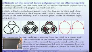
A refined upper bound for the volume...Jones polynomial - Anastasiia Tsvietkova

Anastasiia Tsvietkova, UC Davis October 8, 2015 http://www.math.ias.edu/wgso3m/agenda 2015-2016 Monday, October 5, 2015 - 08:00 to Friday, October 9, 2015 - 12:00 This workshop is part of the topical program "Geometric Structures on 3-Manifolds" which will take place during the 2015-2016

From playlist Workshop on Geometric Structures on 3-Manifolds

Lecture 16: Microarray Disease Classification II

MIT HST.512 Genomic Medicine, Spring 2004 Instructor: Dr. Steven A. Greenberg View the complete course: https://ocw.mit.edu/courses/hst-512-genomic-medicine-spring-2004/ YouTube Playlist: https://www.youtube.com/watch?v=_-gQchCLmXk&list=PLUl4u3cNGP613PJMNmRjAIdBr76goU1V5 I thought what w

From playlist MIT HST.512 Genomic Medicine, Spring 2004

Complex Numbers Exam Review (3 of 4: Cube roots of unity)

More resources available at www.misterwootube.com

From playlist Using Complex Numbers

Huyên Pham - Randomization approach for stochastic control problems

Huyên Pham (Université Paris Diderot) We study optimal stochastic control problem for non-Markovian stochastic differential equations (SDEs) where the drift, diffusion coefficients, and gain functionals are path-dependent, and importantly we do not make any ellipticity assumption on the

From playlist Schlumberger workshop on Topics in Applied Probability

CSDM - Chaim Even Zohar - October 6, 2015

http://www.math.ias.edu/calendar/event/83624/1444141800/1444149000

From playlist Computer Science/Discrete Mathematics

What is the amplitude of a trigonometric graph

From playlist How to Graph Trigonometric Functions

Coefficient diagram method

Related pages